Installing and so on

%load_ext autoreload
%autoreload 2

Do a uv sync --extra examples to install the required dependencies

import sys
import os
sys.path.append(os.path.abspath('..'))

from yanat import generative_game_theoric as gen
from yanat import utils as ut
from vizman import viz
import seaborn as sns
import numpy as np
import matplotlib.pyplot as plt
import netneurotools.datasets as nntd
from scipy.spatial.distance import pdist, squareform

For better plots

viz.set_visual_style()

Fetching a human connectome from netneurotools

human_struct = nntd.fetch_famous_gmat("human_struct_scale033")

Please cite the following papers if you are using this function:
  [primary]:

  [celegans]:
    Lav R Varshney, Beth L Chen, Eric Paniagua, David H Hall, and Dmitri B Chklovskii. Structural properties of the caenorhabditis elegans neuronal network. PLoS computational biology, 7(2):e1001066, 2011.
  [drosophila]:
    Ann-Shyn Chiang, Chih-Yung Lin, Chao-Chun Chuang, Hsiu-Ming Chang, Chang-Huain Hsieh, Chang-Wei Yeh, Chi-Tin Shih, Jian-Jheng Wu, Guo-Tzau Wang, Yung-Chang Chen, and others. Three-dimensional reconstruction of brain-wide wiring networks in drosophila at single-cell resolution. Current biology, 21(1):1–11, 2011.
  [human]:
    Alessandra Griffa, Yasser Alemán-Gómez, and Patric Hagmann. Structural and functional connectome from 70 young healthy adults [data set]. Zenodo, 2019.
  [macaque_markov]:
    Nikola T Markov, Maria Ercsey-Ravasz, Camille Lamy, Ana Rita Ribeiro Gomes, Loïc Magrou, Pierre Misery, Pascale Giroud, Pascal Barone, Colette Dehay, Zoltán Toroczkai, and others. The role of long-range connections on the specificity of the macaque interareal cortical network. Proceedings of the National Academy of Sciences, 110(13):5187–5192, 2013.
  [macaque_modha]:
    Dharmendra S Modha and Raghavendra Singh. Network architecture of the long-distance pathways in the macaque brain. Proceedings of the National Academy of Sciences, 107(30):13485–13490, 2010.
  [mouse]:
    Mikail Rubinov, Rolf JF Ypma, Charles Watson, and Edward T Bullmore. Wiring cost and topological participation of the mouse brain connectome. Proceedings of the National Academy of Sciences, 112(32):10032–10037, 2015.
  [rat]:
    Mihail Bota, Olaf Sporns, and Larry W Swanson. Architecture of the cerebral cortical association connectome underlying cognition. Proceedings of the National Academy of Sciences, 112(16):E2093–E2101, 2015.
Dataset ds-famous_gmat already exists. Skipping download.

human_struct.keys()

dict_keys(['labels', 'conn', 'coords', 'dist'])

connectivity = ut.minmax_normalize(human_struct["conn"])
coordinates = human_struct["coords"]

euclidean_distance = squareform(pdist(coordinates))

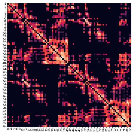
sns.heatmap(connectivity)

<Axes: >

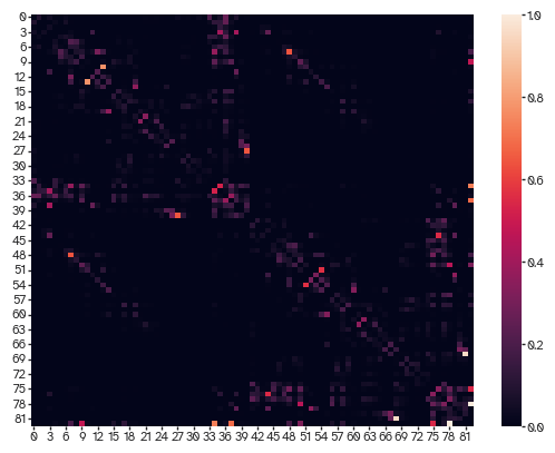
Example of how nodes can have different resources based on empirical data. To be the most parsimonious, you can leave this out. To be more topographically accurate, you can include it. Of course you can define this based on anything else you want e.g., genetics or cytoarchitectonic features.

resource = connectivity.sum(0)/(connectivity.sum(0).max())

The model is fitted to the density of the empirical connectivity matrix:

ut.find_density(connectivity)

np.float64(0.30976919727101176)

Fitting the trade-off parameter:

The model has a coefficient for ‘wiring benefit’ called alpha and one to scale wiring cost called beta. I usually set that to 1 but note that both (and pretty much all other) parameters can be time-varying. Penalty adds a penalty to the payoff for each node, encouraging them to connect to avoid fragmented graphs. This is usually not needed but it can be useful to prevent fragmentation given some metrics. Batch size is the number of nodes to be updated at once so higher means slower computation but faster convergence. Payoff tolerance is the threshold for the change in payoff to be considered worthy. Think of it as a learning rate. If set to zero, it will converge but will continue going through local updates that are driven by numerical noise (in symmetric networks). In directed graphs, and of course given the metric, it converges to a unique solution that is a Nash Equilibrium. To prevent that little fight after convergence in symmetric networks, you can slowly raise the tolerance to make insignificant payoff differences not worthy. Weight is the coefficient of the exponential decay on weights of the generated networks. If this is zero, the networks are evaluated as binary. Otherwise, they’ll get weights based on the euclidean distance with longer connections having exponentially less weight. Resource scaling is the scaling of the resource available to the nodes. Things depend on the metric so you need to find the right balance for these, or leave them out and just go with alpha alone to be the most parsimonious (but also binary). Anyway, let’s try this bad boy:

n_iterations = 3000 # this needs to be higher depending on the metric.
beta_vec = np.ones(n_iterations)
penalty_vec = np.zeros(n_iterations)
batch_size_vec = np.full(n_iterations, 10)
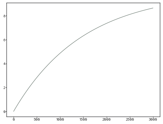
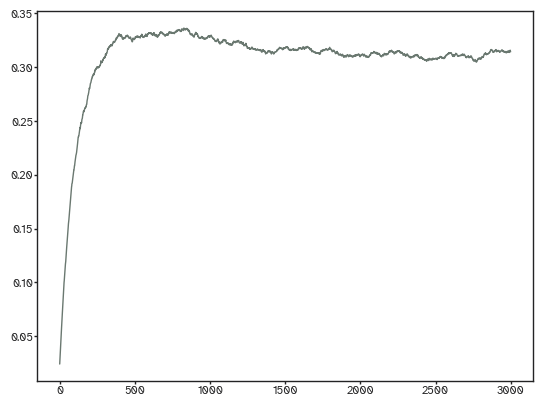
payoff_tolerance_vec = 10 * (1 - np.exp(-2 * np.linspace(0, 1, n_iterations)))
weight = 0.1
resource_scaling = 10

plt.plot(payoff_tolerance_vec)

[<matplotlib.lines.Line2D at 0x16a113850>]

We’ll be using propagation dynamics here with a spatial decay of 0.9. Read here if you want to know more about it: https://doi.org/10.7554/eLife.101780 We use a bisection method to find the optimal alpha with a tolerance of 0.01 difference between the empirical and synthetic density. The maximum number of iterations is 10 and I never exceeded it so far.

result=gen.find_optimal_alpha(
    distance_matrix=euclidean_distance,
    empirical_connectivity=connectivity,
    distance_fn=gen.propagation_distance,
    n_iterations=n_iterations,
    alpha_range=(0.1, 200),
    max_search_iterations=10,
    tolerance=0.01,
    payoff_tolerance=payoff_tolerance_vec,
    batch_size=batch_size_vec,
    node_resources=resource*resource_scaling,
    weight_coefficient=weight,
    spatial_decay = 0.9)

Simulating network evolution:   3%|▎         | 85/2999 [00:06<00:47, 61.28it/s] /Users/kf02/Library/Mobile Documents/com~apple~CloudDocs/Work/Projects/YANAT/YANAT/yanat/utils.py:49: RuntimeWarning: divide by zero encountered in log
  return np.nan_to_num(np.log(adjacency_matrix), neginf=0, posinf=0)
/Users/kf02/Library/Mobile Documents/com~apple~CloudDocs/Work/Projects/YANAT/YANAT/yanat/utils.py:49: RuntimeWarning: divide by zero encountered in log
  return np.nan_to_num(np.log(adjacency_matrix), neginf=0, posinf=0)
/Users/kf02/Library/Mobile Documents/com~apple~CloudDocs/Work/Projects/YANAT/YANAT/yanat/utils.py:49: RuntimeWarning: divide by zero encountered in log
  return np.nan_to_num(np.log(adjacency_matrix), neginf=0, posinf=0)
/Users/kf02/Library/Mobile Documents/com~apple~CloudDocs/Work/Projects/YANAT/YANAT/yanat/utils.py:49: RuntimeWarning: divide by zero encountered in log
  return np.nan_to_num(np.log(adjacency_matrix), neginf=0, posinf=0)
/Users/kf02/Library/Mobile Documents/com~apple~CloudDocs/Work/Projects/YANAT/YANAT/yanat/utils.py:49: RuntimeWarning: divide by zero encountered in log
  return np.nan_to_num(np.log(adjacency_matrix), neginf=0, posinf=0)
/Users/kf02/Library/Mobile Documents/com~apple~CloudDocs/Work/Projects/YANAT/YANAT/yanat/utils.py:49: RuntimeWarning: divide by zero encountered in log
  return np.nan_to_num(np.log(adjacency_matrix), neginf=0, posinf=0)
/Users/kf02/Library/Mobile Documents/com~apple~CloudDocs/Work/Projects/YANAT/YANAT/yanat/utils.py:49: RuntimeWarning: divide by zero encountered in log
  return np.nan_to_num(np.log(adjacency_matrix), neginf=0, posinf=0)
/Users/kf02/Library/Mobile Documents/com~apple~CloudDocs/Work/Projects/YANAT/YANAT/yanat/utils.py:49: RuntimeWarning: divide by zero encountered in log
  return np.nan_to_num(np.log(adjacency_matrix), neginf=0, posinf=0)
/Users/kf02/Library/Mobile Documents/com~apple~CloudDocs/Work/Projects/YANAT/YANAT/yanat/utils.py:49: RuntimeWarning: divide by zero encountered in log
  return np.nan_to_num(np.log(adjacency_matrix), neginf=0, posinf=0)
/Users/kf02/Library/Mobile Documents/com~apple~CloudDocs/Work/Projects/YANAT/YANAT/yanat/utils.py:49: RuntimeWarning: divide by zero encountered in log
  return np.nan_to_num(np.log(adjacency_matrix), neginf=0, posinf=0)
Simulating network evolution:   3%|▎         | 94/2999 [00:06<00:43, 67.11it/s]/Users/kf02/Library/Mobile Documents/com~apple~CloudDocs/Work/Projects/YANAT/YANAT/yanat/utils.py:49: RuntimeWarning: divide by zero encountered in log
  return np.nan_to_num(np.log(adjacency_matrix), neginf=0, posinf=0)
/Users/kf02/Library/Mobile Documents/com~apple~CloudDocs/Work/Projects/YANAT/YANAT/yanat/utils.py:49: RuntimeWarning: divide by zero encountered in log
  return np.nan_to_num(np.log(adjacency_matrix), neginf=0, posinf=0)
/Users/kf02/Library/Mobile Documents/com~apple~CloudDocs/Work/Projects/YANAT/YANAT/yanat/utils.py:49: RuntimeWarning: divide by zero encountered in log
  return np.nan_to_num(np.log(adjacency_matrix), neginf=0, posinf=0)
/Users/kf02/Library/Mobile Documents/com~apple~CloudDocs/Work/Projects/YANAT/YANAT/yanat/utils.py:49: RuntimeWarning: divide by zero encountered in log
  return np.nan_to_num(np.log(adjacency_matrix), neginf=0, posinf=0)
/Users/kf02/Library/Mobile Documents/com~apple~CloudDocs/Work/Projects/YANAT/YANAT/yanat/utils.py:49: RuntimeWarning: divide by zero encountered in log
  return np.nan_to_num(np.log(adjacency_matrix), neginf=0, posinf=0)
/Users/kf02/Library/Mobile Documents/com~apple~CloudDocs/Work/Projects/YANAT/YANAT/yanat/utils.py:49: RuntimeWarning: divide by zero encountered in log
  return np.nan_to_num(np.log(adjacency_matrix), neginf=0, posinf=0)
Simulating network evolution: 100%|██████████| 2999/2999 [00:42<00:00, 70.80it/s]
Simulating network evolution: 100%|██████████| 2999/2999 [00:37<00:00, 79.87it/s]

Initial range: alpha=[0.1, 200], density=[0.0005877167205406994, 0.39288862768145755]
Target density: 0.31354687040846313
Iteration 1: Testing alpha=159.57078651685393

Simulating network evolution: 100%|██████████| 2999/2999 [00:37<00:00, 79.87it/s]

Alpha=159.57078651685393 → density=0.3643843667352336, diff from target=0.05083749632677048
Iteration 2: Testing alpha=137.28609664010457

Simulating network evolution: 100%|██████████| 2999/2999 [00:38<00:00, 78.71it/s]

Alpha=137.28609664010457 → density=0.35027916544225685, diff from target=0.036732295033793716
Iteration 3: Testing alpha=122.87579237118602

Simulating network evolution: 100%|██████████| 2999/2999 [00:39<00:00, 75.24it/s]

Alpha=122.87579237118602 → density=0.3379371143109021, diff from target=0.02439024390243899
Iteration 4: Testing alpha=113.99914536177101

Simulating network evolution: 100%|██████████| 2999/2999 [00:42<00:00, 70.43it/s]

Alpha=113.99914536177101 → density=0.3253012048192771, diff from target=0.011754334410813971
Iteration 5: Testing alpha=109.87609937582457

Simulating network evolution: 100%|██████████| 2999/2999 [00:40<00:00, 74.62it/s]

Alpha=109.87609937582457 → density=0.3241257713781957, diff from target=0.010578900969732574
Iteration 6: Testing alpha=106.28669013192841

Simulating network evolution: 100%|██████████| 2999/2999 [00:37<00:00, 78.97it/s]

Alpha=106.28669013192841 → density=0.3182486041727887, diff from target=0.0047017337643255885

result.keys()

dict_keys(['alpha', 'density', 'evolution'])

result["evolution"].shape

(83, 83, 3000)

from scipy.stats import spearmanr

weighted_adj = np.zeros_like(result["evolution"])
for network in range(result["evolution"].shape[-1]):
    weighted_adj[...,network] = gen._apply_weighting(result["evolution"][...,network],euclidean_distance,weight)

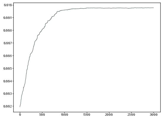
plt.plot(weighted_adj.mean((0,1)))

[<matplotlib.lines.Line2D at 0x17f44b610>]

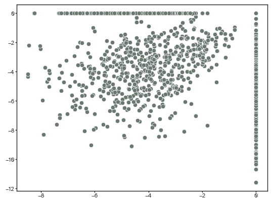
sns.scatterplot(x=ut.log_normalize(weighted_adj[...,-1]).flatten(),
 y=ut.log_normalize(connectivity).flatten())

/Users/kf02/Library/Mobile Documents/com~apple~CloudDocs/Work/Projects/YANAT/YANAT/yanat/utils.py:49: RuntimeWarning: divide by zero encountered in log
  return np.nan_to_num(np.log(adjacency_matrix), neginf=0, posinf=0)

<Axes: >

spearmanr(weighted_adj[...,-1].flatten(),connectivity.flatten())

SignificanceResult(statistic=np.float64(0.44798373001772485), pvalue=np.float64(0.0))

This might seem good but I usually test against the value we get just from the euclidean distance.

spearmanr(euclidean_distance.flatten(),connectivity.flatten())

SignificanceResult(statistic=np.float64(-0.4061853909430151), pvalue=np.float64(5.312447132311121e-272))

So, a bit better!

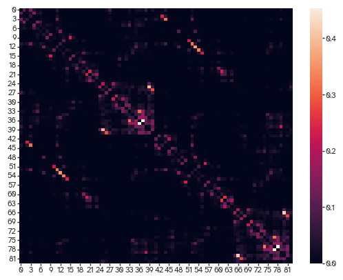
sns.heatmap(weighted_adj[...,-1])

<Axes: >

viz.plot_matrix(ut.log_minmax_normalize(weighted_adj[...,-1]))

/Users/kf02/Library/Mobile Documents/com~apple~CloudDocs/Work/Projects/YANAT/YANAT/yanat/utils.py:49: RuntimeWarning: divide by zero encountered in log
  return np.nan_to_num(np.log(adjacency_matrix), neginf=0, posinf=0)

<Axes: >

densities = [ut.find_density(result["evolution"][...,i]) for i in range(result["evolution"].shape[-1])]

plt.plot(densities);

If you have a bunch of empirical networks with the same density, then all you have to do is to use the same parameters to generate synthetic ones. That optimization function is just calling this one under the hood. Here’s how to make one:

nets = gen.simulate_network_evolution(
            distance_matrix=euclidean_distance,
            n_iterations=n_iterations,
            distance_fn=gen.propagation_distance,
            alpha=result["alpha"],
            beta=beta_vec,
            connectivity_penalty=penalty_vec,
            n_jobs=-1,
            random_seed=11,
            batch_size=batch_size_vec,
            payoff_tolerance=payoff_tolerance_vec,
            weight_coefficient=weight,
            node_resources=resource*resource_scaling,
            spatial_decay = 0.9
        )

Simulating network evolution: 100%|██████████| 2999/2999 [00:41<00:00, 71.60it/s]

densities = [ut.find_density(nets[...,i]) for i in range(nets.shape[-1])]

plt.plot(densities);

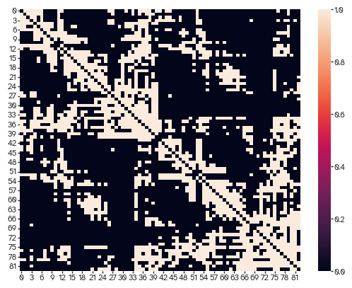
By default, synthetic networks are binary:

sns.heatmap(nets[...,-1])

<Axes: >

We can check how well the degree distributions match.

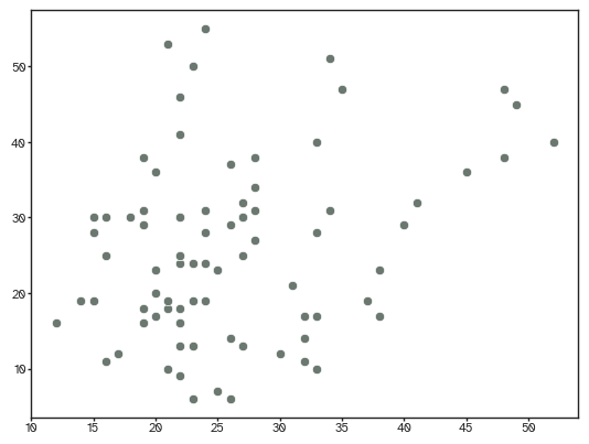
sns.scatterplot(x=nets[..., -1].sum(axis=1),
y=connectivity.astype(bool).astype(int).sum(axis=1))

<Axes: >

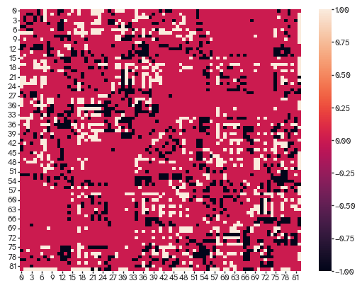
And what stuff is missed

sns.heatmap(connectivity.astype(bool)-nets[...,-1])

<Axes: >

we can also look at the cosine similarity between the two networks to see how similar they are.

from yanat.utils import calculate_endpoint_similarity
calculate_endpoint_similarity(connectivity.astype(bool).astype(int), nets[...,-1]).mean()

np.float64(0.570789557808441)

Not bad actually. But what about the topography, i.e., the spatial distribution of edges

spearmanr(nets[..., -1].sum(axis=1), connectivity.astype(bool).astype(int).sum(axis=1))

SignificanceResult(statistic=np.float64(0.2150308148390282), pvalue=np.float64(0.05091255014113673))

Also not bad but remember the resources have a role here. Anyway, here’s an animation showing the whole wiring battle:

from matplotlib import animation
fig = plt.figure()

ims = []
for i in range(nets.shape[-1]):
    im = plt.imshow(nets[...,i], animated=True)
    ims.append([im])

ani = animation.ArtistAnimation(fig, ims, interval=200, blit=True,
                                repeat_delay=100)
from IPython.display import HTML
HTML(ani.to_jshtml())

Animation size has reached 20983227 bytes, exceeding the limit of 20971520.0. If you're sure you want a larger animation embedded, set the animation.embed_limit rc parameter to a larger value (in MB). This and further frames will be dropped.

Once Loop Reflect